 Nima Leclerc
Explained · 06 · Paper · ICML 2026
When is it worth tuning each quantum device separately?
A scaling law that predicts how much a controller gains from adapting to an individual chip, and when the effort is wasted.
The problem
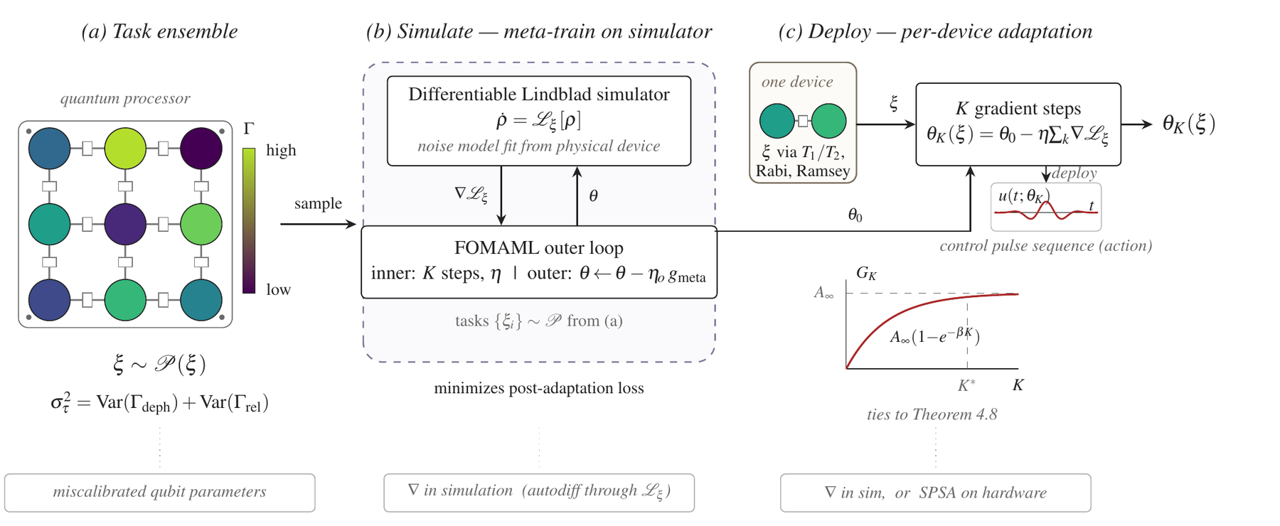
Quantum computers have to be recalibrated, constantly. No two chips are identical, and each one drifts over hours. On large machines the daily calibration can take an hour or more, and that cost grows as the number of qubits does. Engineers face a choice. Use one fixed, “robust” control pulse that is good enough everywhere, or spend time tuning pulses for each device. Until now there was no quantitative guide for when the second option pays off.
The approach
We treat each device as a “task”, a particular set of noise rates and coherence times. We train a meta-initialization, a starting point for the control pulse learned across many simulated devices. At deployment, a few gradient steps specialize it to the actual device. The gain from those steps is the adaptation gain.
The scaling law
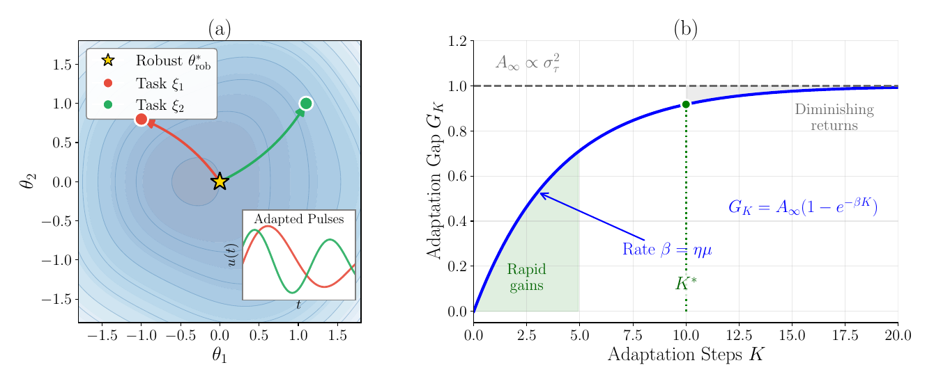
We derive a lower bound on that gain. It has a simple form: the gain rises with the number of adaptation steps K and then saturates exponentially, following GK = A∞(1 − e−βK), and the ceiling A∞ scales linearly with how much the devices differ from one another (the task variance). In plain terms: if all your devices are alike, a single robust pulse is nearly as good as tuning each one. If they differ a lot, tuning pays, with diminishing returns after the first few steps.
Does it hold up?
- On tasks with low variation between devices, adaptation gives negligible benefit, as the law predicts.
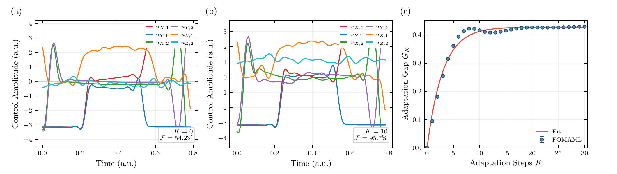
- On a two-qubit CZ gate under extreme noise (10× what the controller trained on), adaptation lifts the gate fidelity from 54% to 96% after 10 steps, a gain of more than 40 percentage points, and the measured curve fits the predicted exponential.
- The same law appears in a classical linear-quadratic control problem, which suggests it comes from the geometry of the optimization rather than from quantum physics in particular.
A practical rule of thumb
We also give a few-shot protocol: run just 3 to 5 probe steps on a new device, and use them to estimate how many steps are worth spending, to within 3–19% relative error across the out-of-distribution cases we tried.
The limits
The study is in simulation, assumes noise statistics that stay constant during a run, and uses a differentiable model of the device. Drifting noise within a run would need an online version. But the result gives practitioners a number to reason with instead of a hunch.